In Part 1 we explained how to add different base map layers to QGIS allowing us to bring up different geographic views. In this second part we ll download and overlay various geographical and outdoor features from Open Street Maps to allow us to plan a Himalayan traverse.
Contents
- Open Street Maps
- QuickOSM Plugin
- Major valleys / Rivers
- Minor valleys/ Streams
- Mountain passes
- Mountain peaks
Open Street Maps
OpenStreetMap (OSM) is a free, open geographic database updated and maintained by a community of volunteers via open collaboration. Contributors collect data from surveys, trace from aerial imagery and also import from other freely licensed geodata sources. The outdoor community has extensively mapped the geography of the Himalayas (river and valleys) as well as various outdoor features like hiking routes, mountain passes, campsites, settlements, shelters, etc.
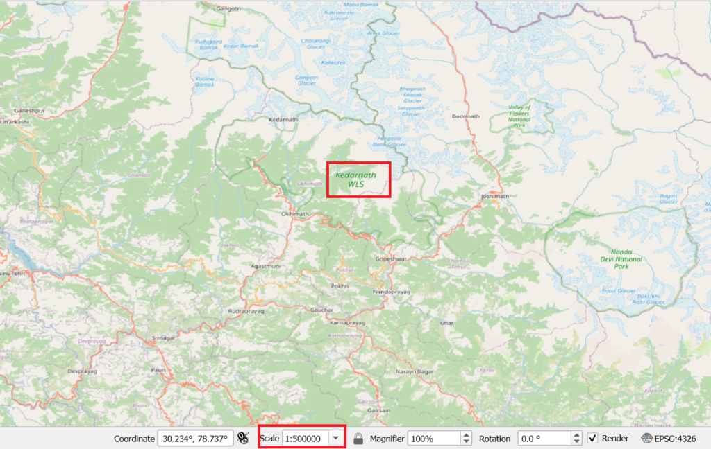
Let’s analyze the geography of Uttarakhand centered around Kedarnath WLS (type in Coordinate window: 30.52, 79.2) at a scale of 1:500K.
If you have trouble finding this region simply download this window extent and drag-n-drop the GPX file into QGIS.
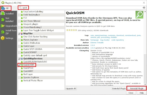
To download data from OSM we install the QGIS QuickOSM plug-in
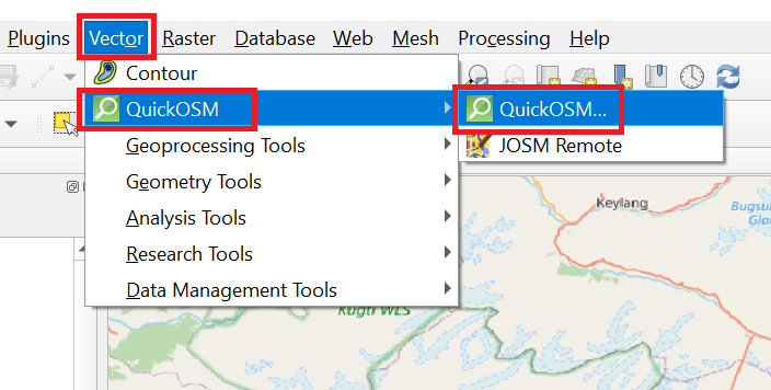
Bring up the QuickOSM query window via the Vector – QuickOSM menu
Major Valleys
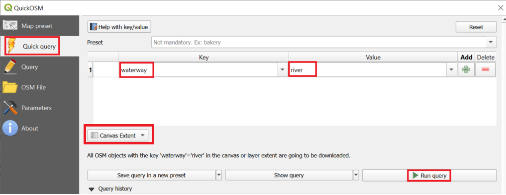
Let’s first retrieve the major valleys (rivers) to get a better understanding of the Himalayan geography. OSM data can be queried using (key, value) pairs as documented in the Open Street Map Wiki. For major rivers we can use “waterway=river”. Ensure to select “Canvas Extent” to download features for the current map view only.
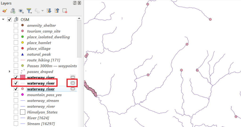
Three new vector layers “waterway_river” are created – a polygon, line and point layer. Delete the polygon and point layers and keep the line layer
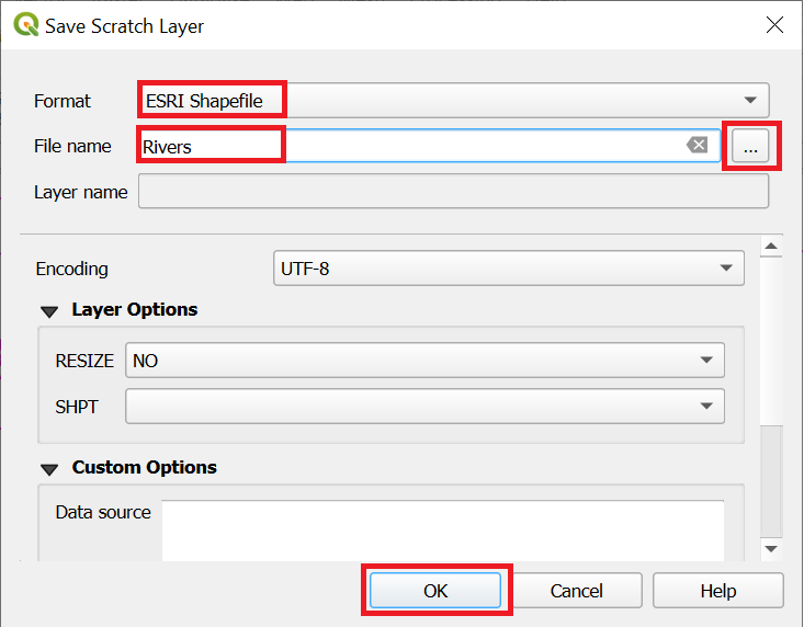
Save the line vector layer by clicking on the chip icon next to the name and save as “ESRI Shapefile” format. Important: click on “…” right of the File Name and ensure to save the file in a directory for which you have write permission on your system.
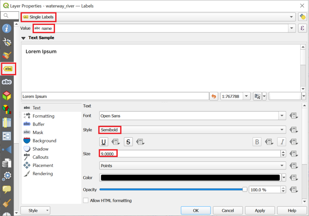
Let’s now visualize the rivers a bit more appropriate. Right click on the line “waterway_river” layer and select Properties. Select the “Labels” tab and select “Single Labels”, “Value=name”, “Size=9”, “Style=Semibold”
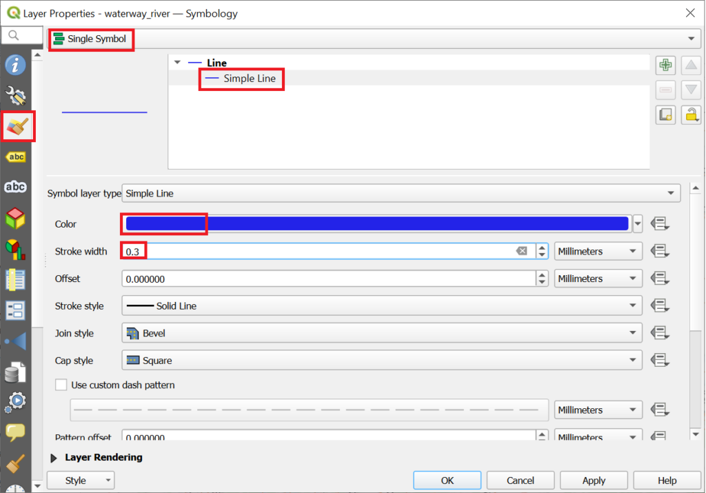
Select the “Symbology” tab, set “Color=blue” and “Stroke Width=0.3”
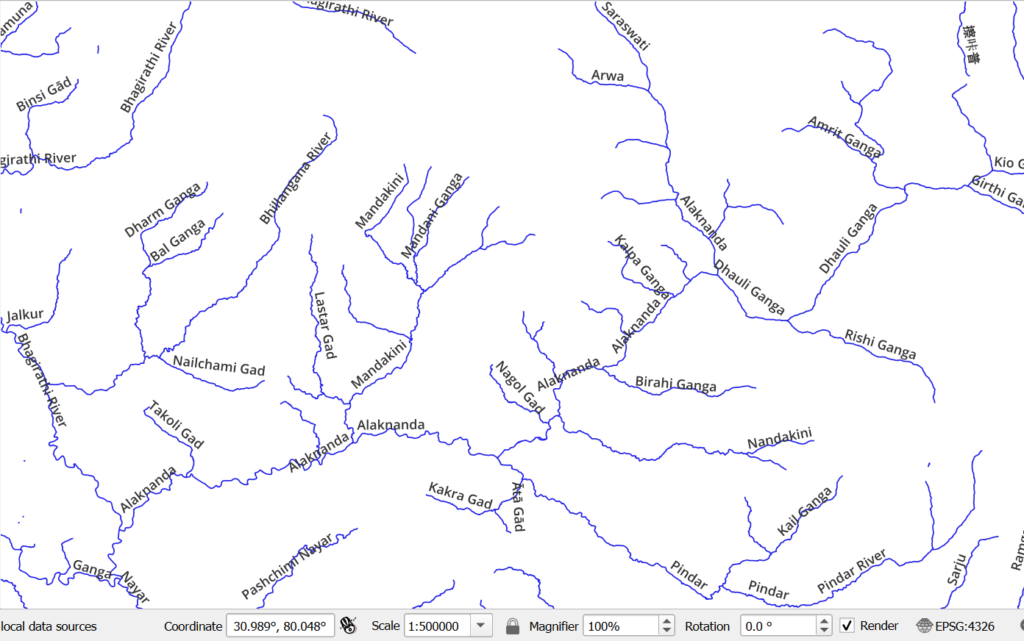
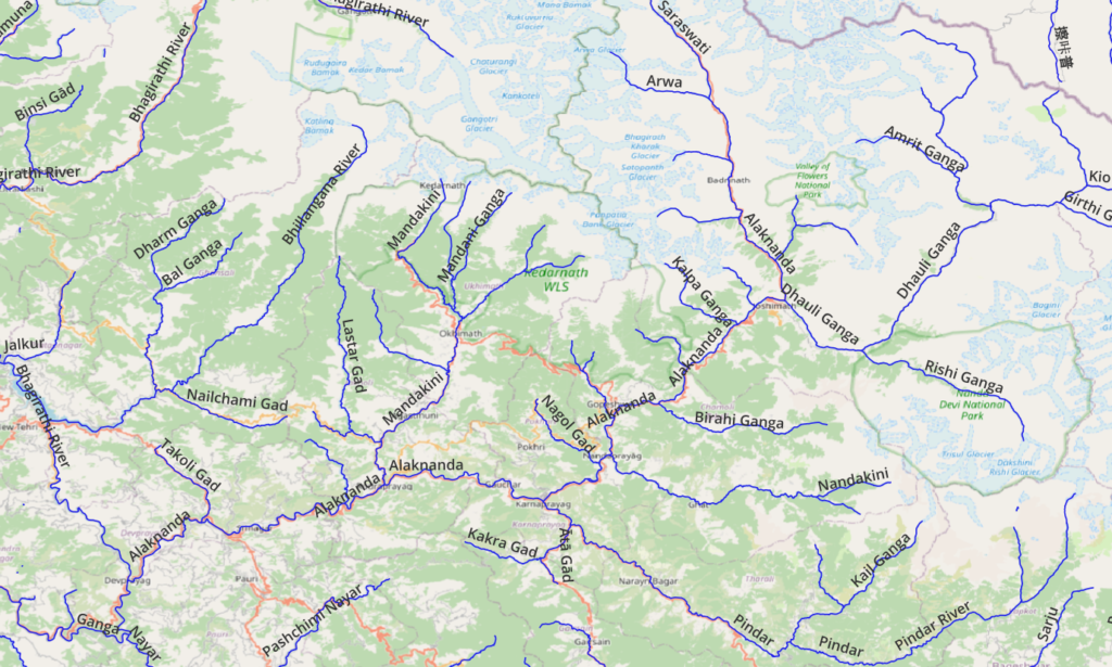
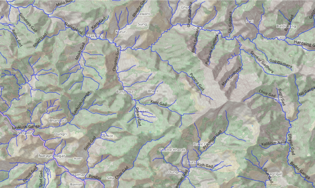
This will show all rivers (major valleys) in blue along with the name
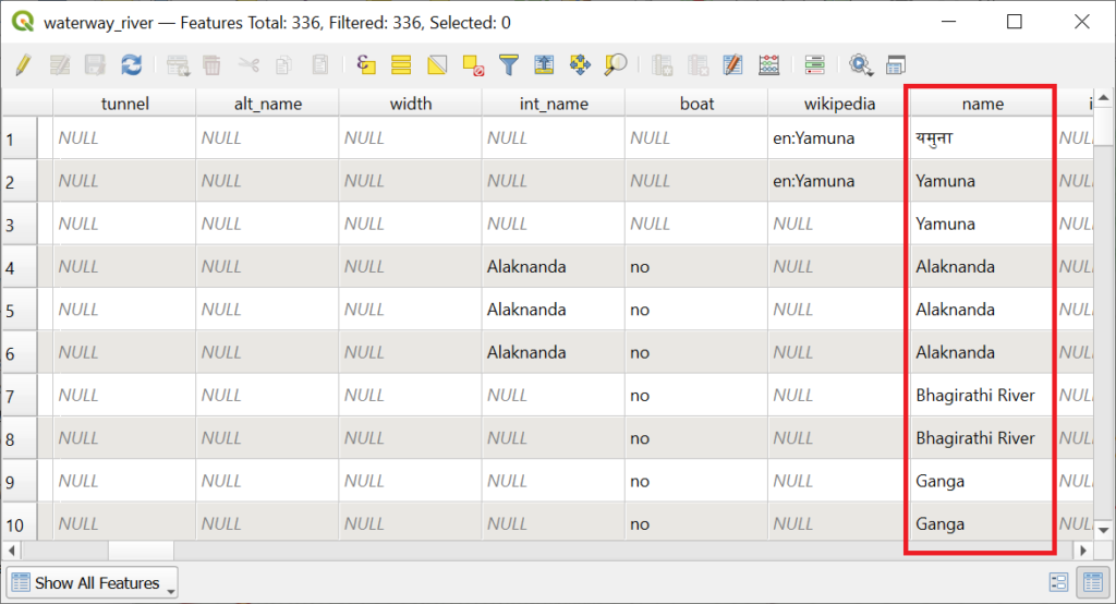
Choose “Open Attributes Table” on the vector layer to get a tabular view on all the rivers. The “name” attribute lists the various river names
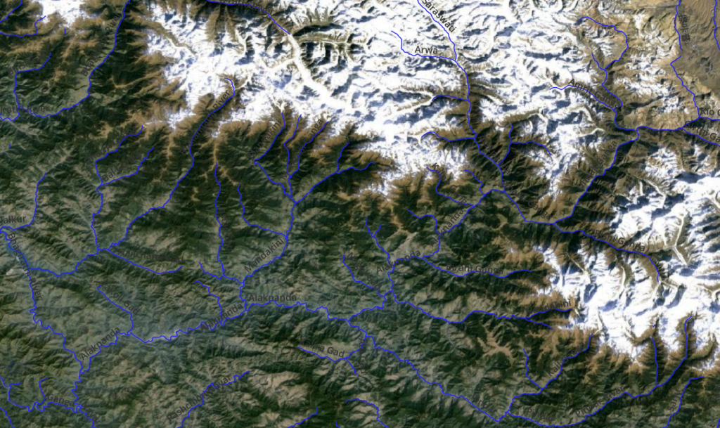
The same geography can be visualized on top of any basemap like Satellite or OSM to add terrain details
Minor Valleys
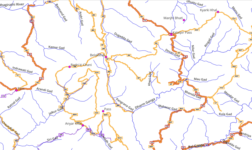
Zoom back to the original center (30.52, 79.2) at 1:500K scale and repeat the above process using “waterway=stream” to bring up minor valleys in the geography. Save the line vector layer and set Label and Symbology
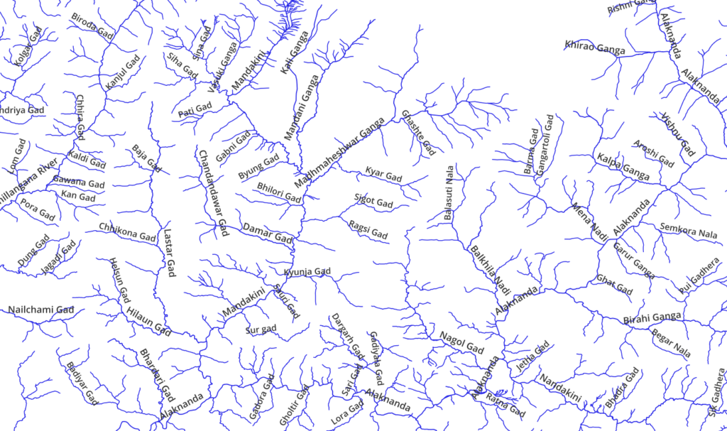
Overlaying the major / minor valleys over a topographic layer like Thunderforest Landscape shows how rivers and stream drain rain, snow and glacial melt from the Himalayan geography
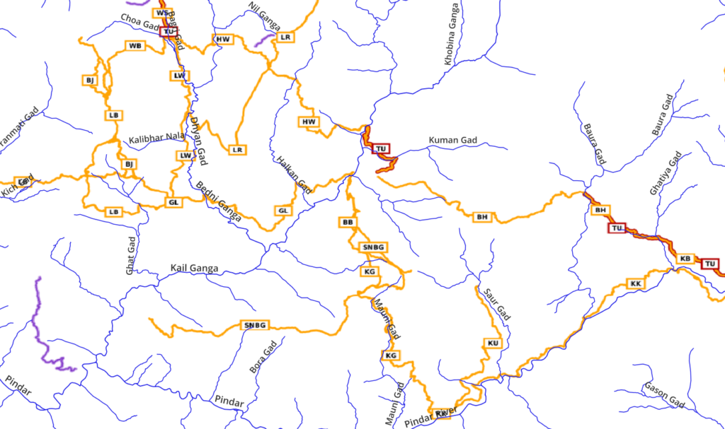
Overlaying the “Waymarked Hiking Trails” layer visualizes how the OSM hiking routes connect various major and minor valleys. This is also useful to identify drinking water points.
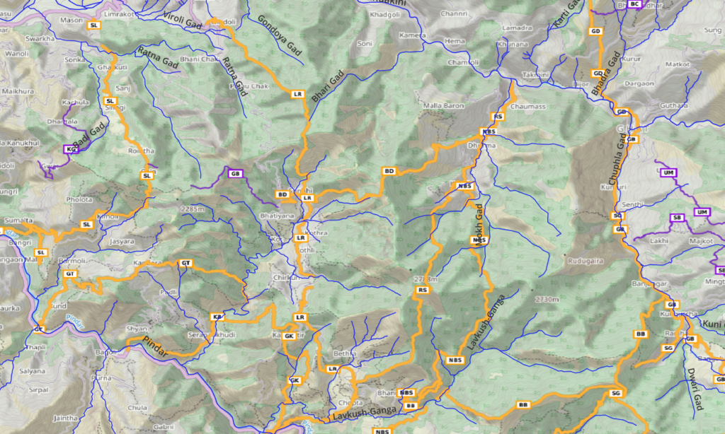
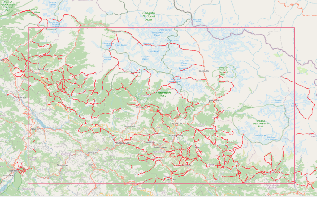
Overlaying topography + geography + hiking routes illustrates how the hiking routes extend across the Himalayan topography
Mountain Passes
Mountain passes are the high points where hiking routes cross over a mountain range or ridgeline connecting neighboring valleys. Zoom back to the original center (330.52, 79.2) at 1:500K scale. We can query the same from OSM using the “mountain_pass=yes” (key, value) pair
View “Open Attributes Table” to get a tabular listing
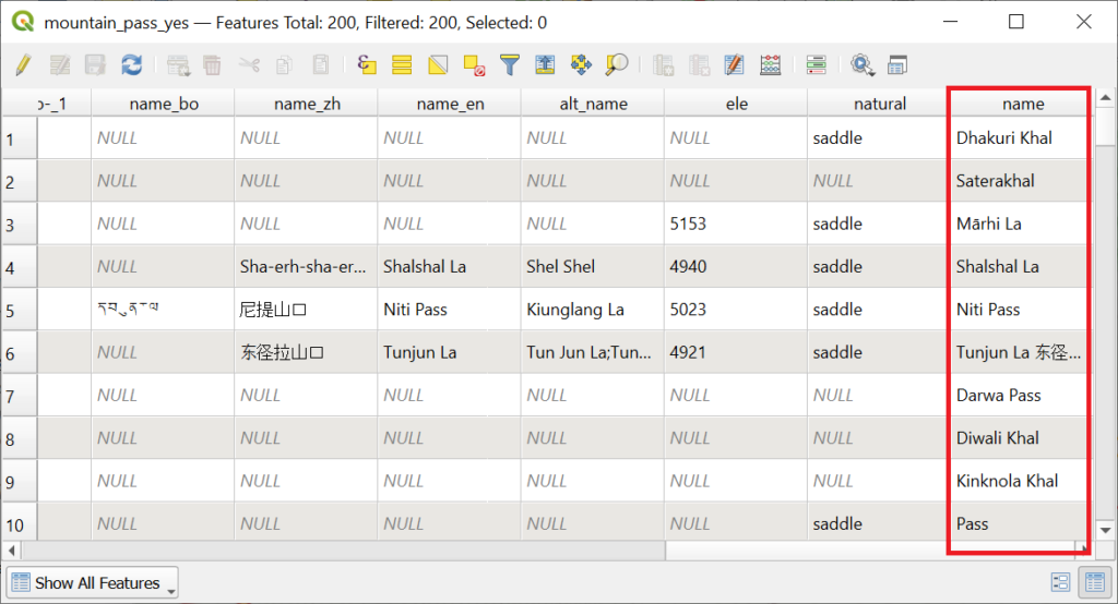
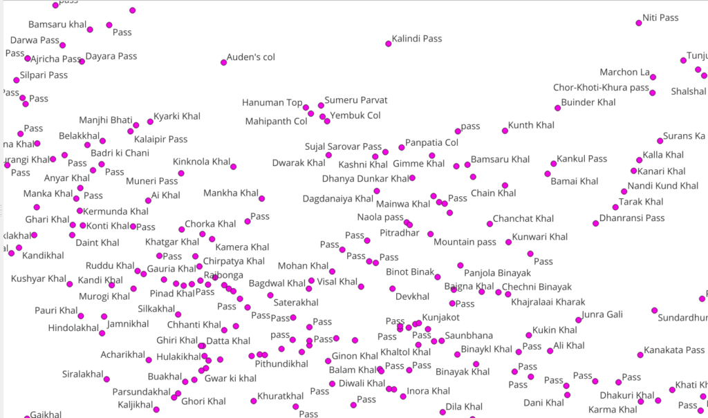
We see that mountain passes are located on the mountain ranges and ridgelines between the valleys (rivers). Mountain passes are shortcuts for the shepherds and locals to commute between neighboring valleys.
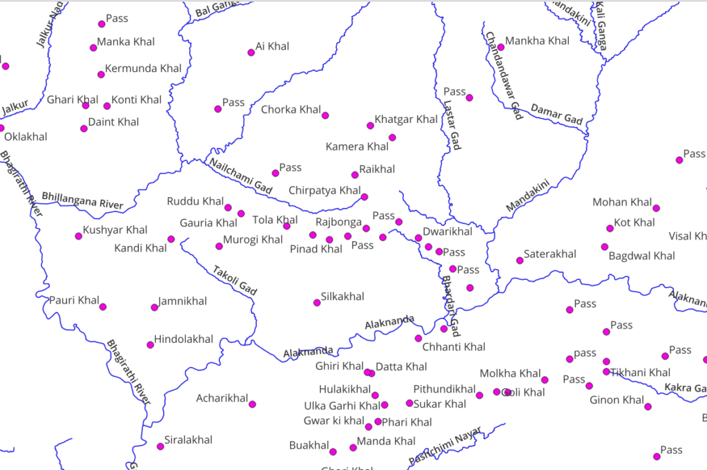
Overlay mountain passes on Open Street Maps to visualize their location in the Himalayan geography
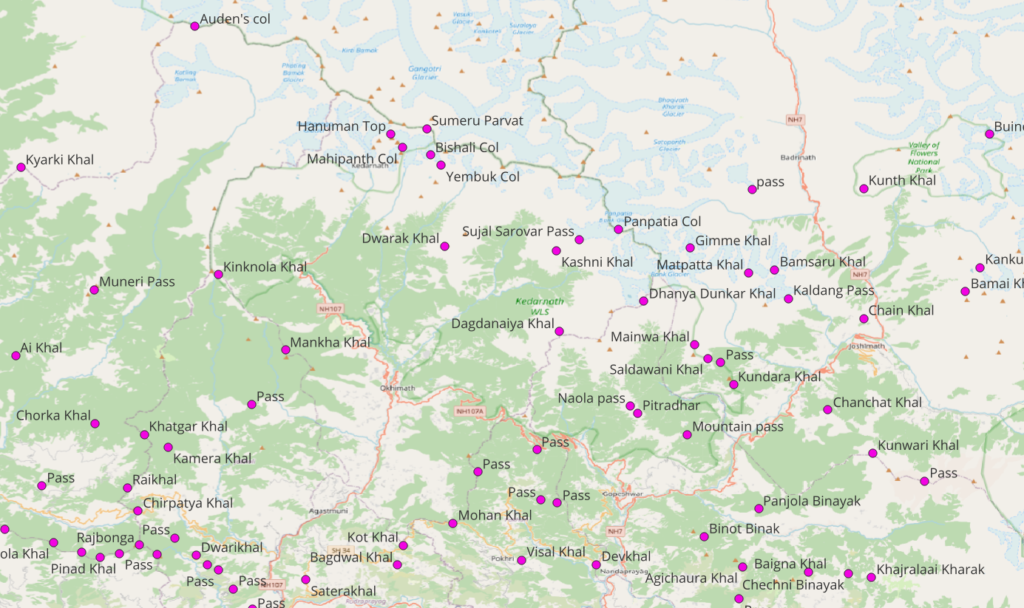
Overlay a topographic map + hiking routes + passes to see how hiking routes cross over high ranges through mountain passes
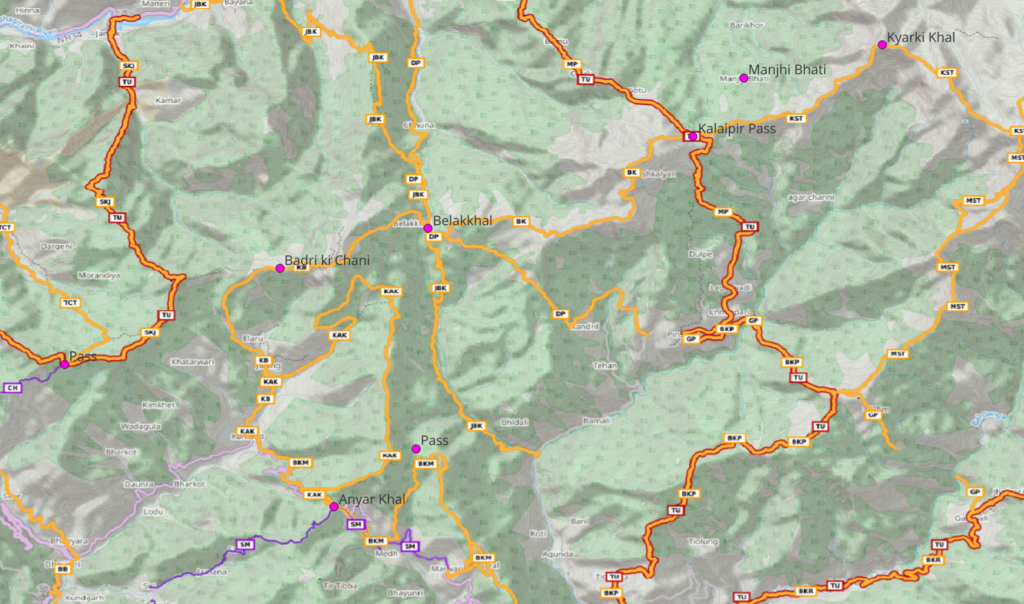
Overlay mountain passes + valleys + hiking routes to see how hiking routes connect neighboring valleys via mountain passes
Mountain Peaks
Another interesting outdoor feature to visualize are mountain peaks. Zoom back to the original center (30.52, 79.2) at 1:500K scale. Download “natural=peak” from OSM to download the same
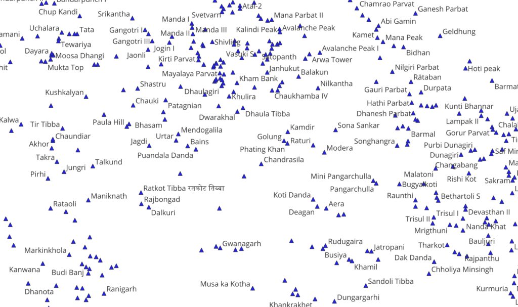
Mountain peaks correspond to the highest points in the topography
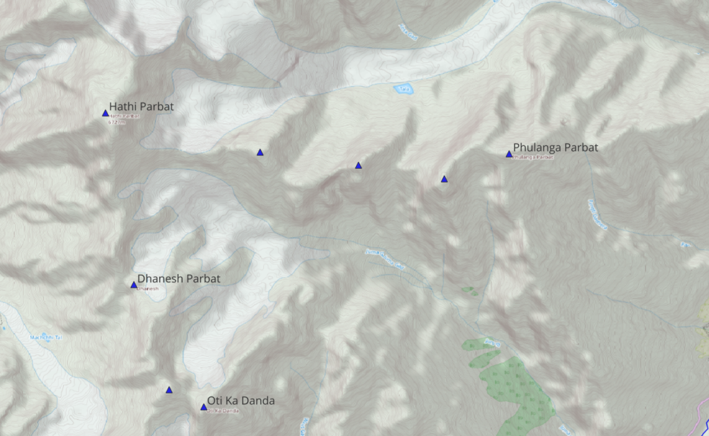
Overlaying OSM base map + peaks + hiking routes visualizes which hiking routes might touch or give a clear view on some nearby peaks

In part 3 we will start planning Himalayan traverses via continuous hiking routes across multiple mountain passes planning for food supply in nearby settlements and night halt in camp sites and shelters.
Assignments
Calculate the total distance of OSM hiking routes around the Kedarnath WLS
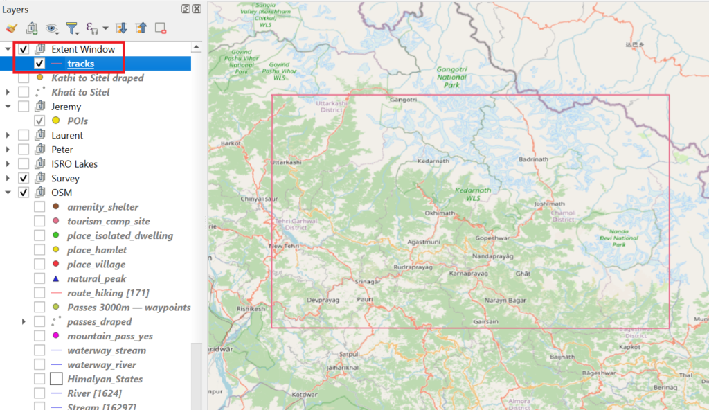
- Make your map view equal to this extent
- Or simply zoom back to (30.52, 79.2) at 1:500K scale
- Set the map scale as 1:500K
- Download OSM “route=hiking”
- Bring up Attribute Table
- Use Expression Editor in Select Features
- Formula: “sum($length)” – the sum of length of each hiking route
- Total length is shown on the bottom
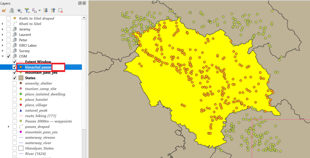
Calculate the total number of mountain passes in the state of Himachal
- Show entire state of Himachal in the map view
- Download state boundaries
- boundary=administrative
- admin_level=4
- Himachal and neighboring states will be downloaded
- “Toggle Edit” on the newly downloaded polygon vector layer
- Use the “Select Features” tool to select and remove all other states
- Keep only the state of Himachal
- View the entire state of Himachal
- Download all “mountain_pass=yes”
- Choose “Vector”, “Geoprocessing Tools”, “Intersection”
- Intersect the downloaded mountain passes with the vector layer containing the boundary of Himachal
- Bring up the “Attributes Table” of the intersection and count the number of passes