
In this chapter we will explore the powerful geometry processing capabilities of QGIS on various Himalayan features. These capabilities will assist the alpine style hiker in more sophisticated terrain analysis and more detailed planning of his journeys throughout the seasons and geography:
Module 1 – Mountain passes (elevation)
Module 2 – Alpine lakes (elevation, area)
Module 3 – Rivers (length, profile, origin, tree hierarchy)
Module 4 – Settlements (type, elevation, terrain)
Module 5 – Hiking routes (length, profile, proximity)
Module 6 – Topography (features, steepness, slope direction)
In this module we will play around with mountain passes (from Open Street Maps) in the state of Himachal Pradesh and visualize / classify them as per their altitude using DEM (from SRTM).
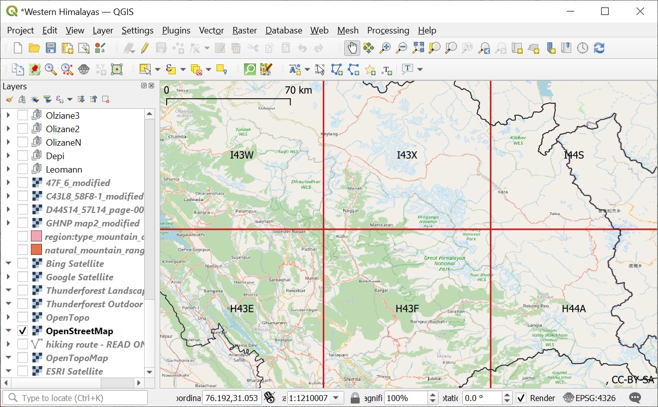
Open up QGIS, set an OpenStreetMap base layer and zoom onto the state of Himachal Pradesh. See image 1 below.
Himachal Pradesh shown in the QGIS main window (red lines = degree boundaries are just shown for reference)
Downloading DEM
Let’s start by downloading DEM (Digital Elevation Model) data for Himachal which we will use to determine the elevation of various Himalayan features in various modules of this chapter. Ensure the QGIS Plug-in “SRTM Downloader” is installed and proper login credentials are configured (refer module 6E).
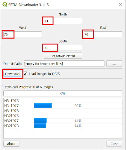
Select “SRTM Downloader” from the QGIS “Plug-ins” menu and download DEM for the region latitude, longitude – 76 East, 31 North to 79 East, 33 North which covers most of HP. This will download 6 data sets, each covering 1×1 degrees or 111x111km. See Image 1 below
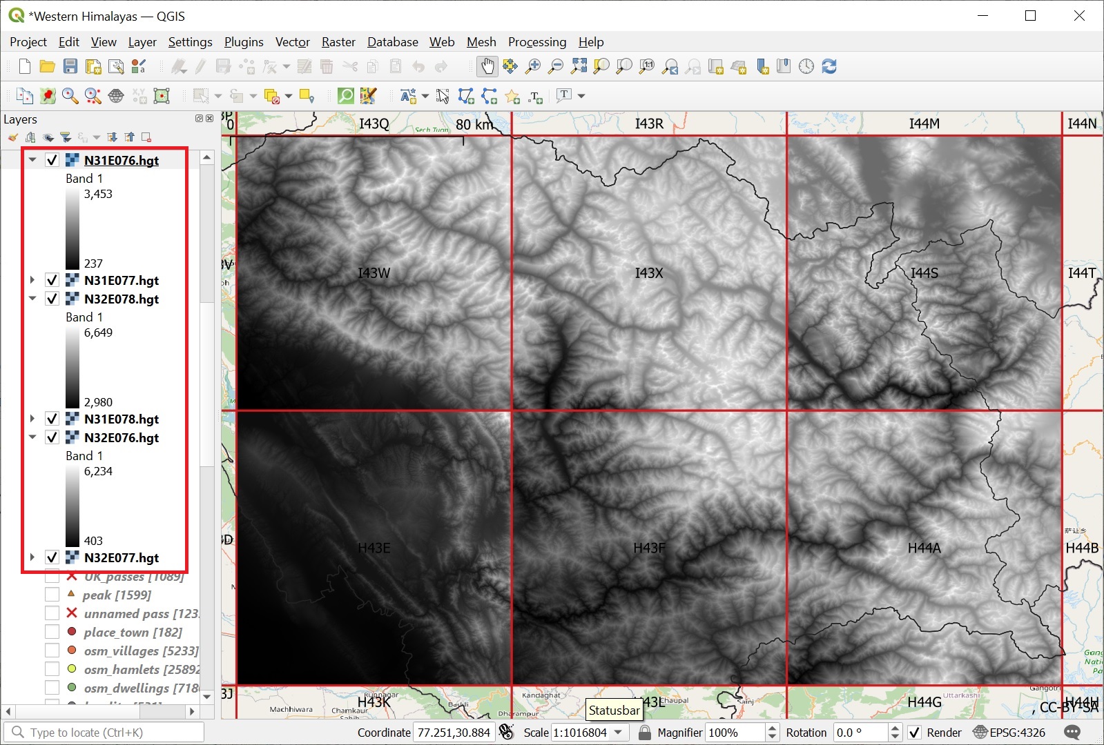
After the download completes, 6 raster layers will be added to QGIS each one having a different gray scale from black (minimum elevation) to white (maximum elevation) for that specific 1×1 degree square. See Image 2 below.
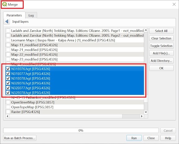
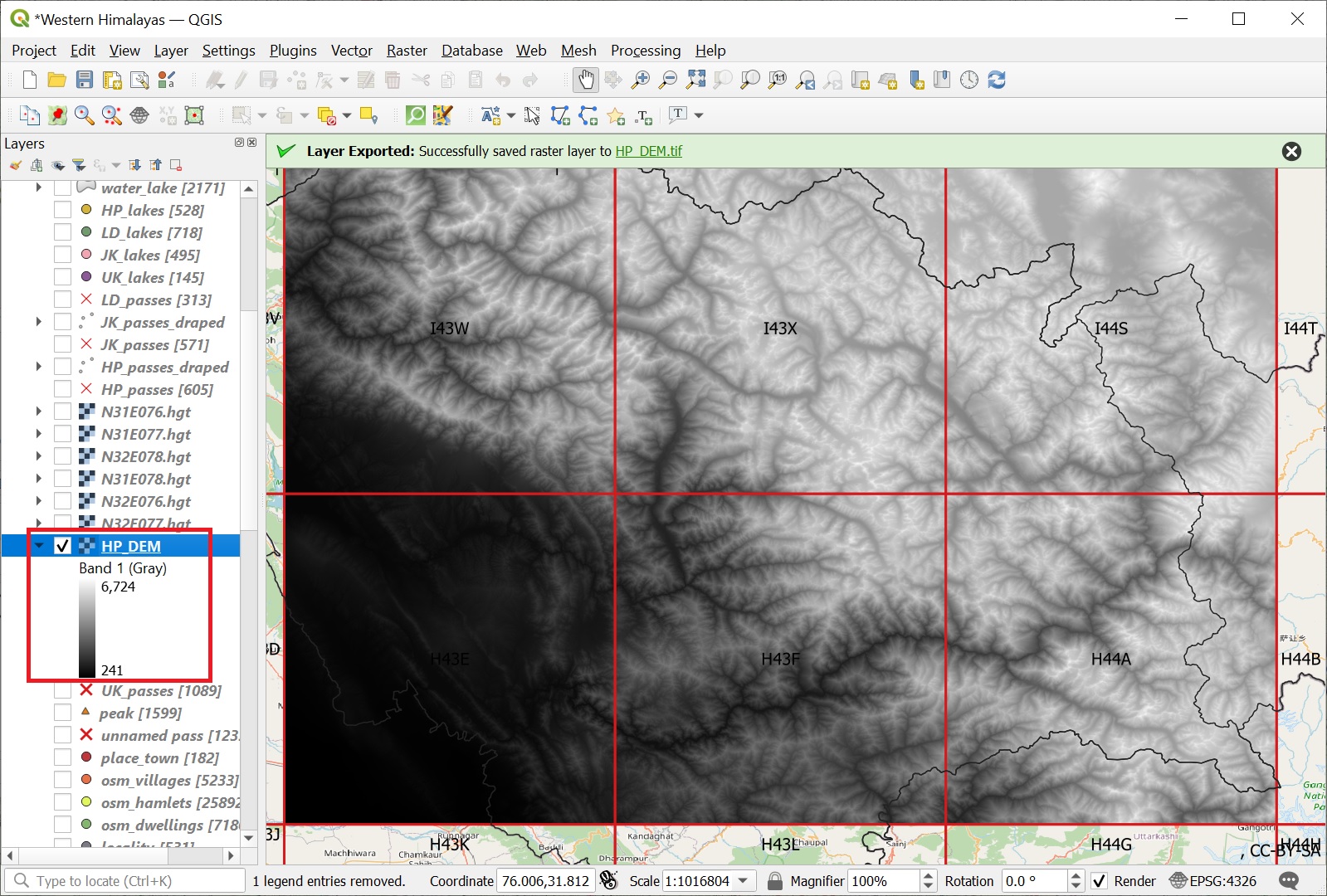
Next, choose QGIS menu “Raster”, “Miscellaneous”, “Merge” to merge the 6 raster layers into one layer with uniform gray scale – min elevation 241m (black) to max elevation 6724 (white). See Image 3 below.
Export the merged raster layer as a GeoTIFF file named as “HP_DEM” (around 300MB in size). See Image 4 below.Downloading DEM for Himachal Pradesh
Six raster layers containing SRTM DEM data for 1×1 degree squares
Merging 6 DEM raster layers
Merged DEM raster layer covering most of Himachal Pradesh
Exporting the merged raster layer as a GeoTIFF file

Mountain Passes
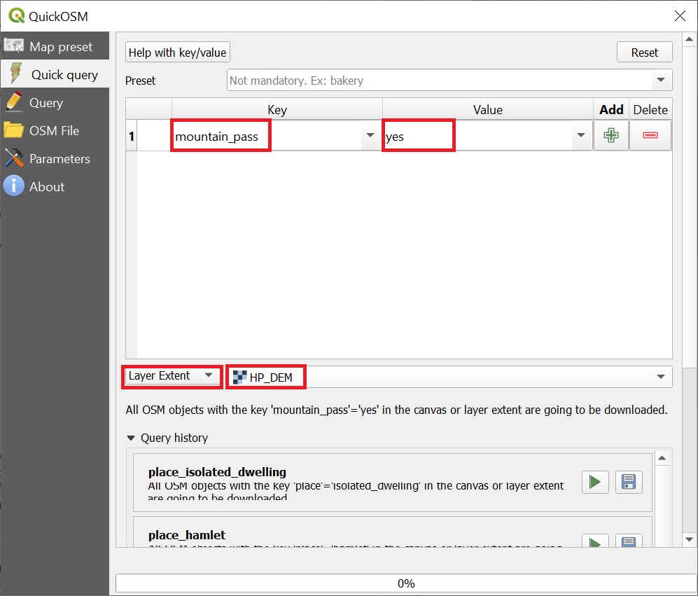
Now let’s query the mountain passes for the same region from Open Street Maps. Ensure the QGIS Plug-in “Quick OSM” is properly installed (refer module 6C). Click on the QuickOSM icon on the toolbar (Select QGIS “View” menu, “Toolbars”, “QuickOSM” to shown toolbar) and query for “mountain_pass” = “yes” for “Layer Extent” = “HP_DEM” (same area covered by our downloaded DEM data). See Image 1 below
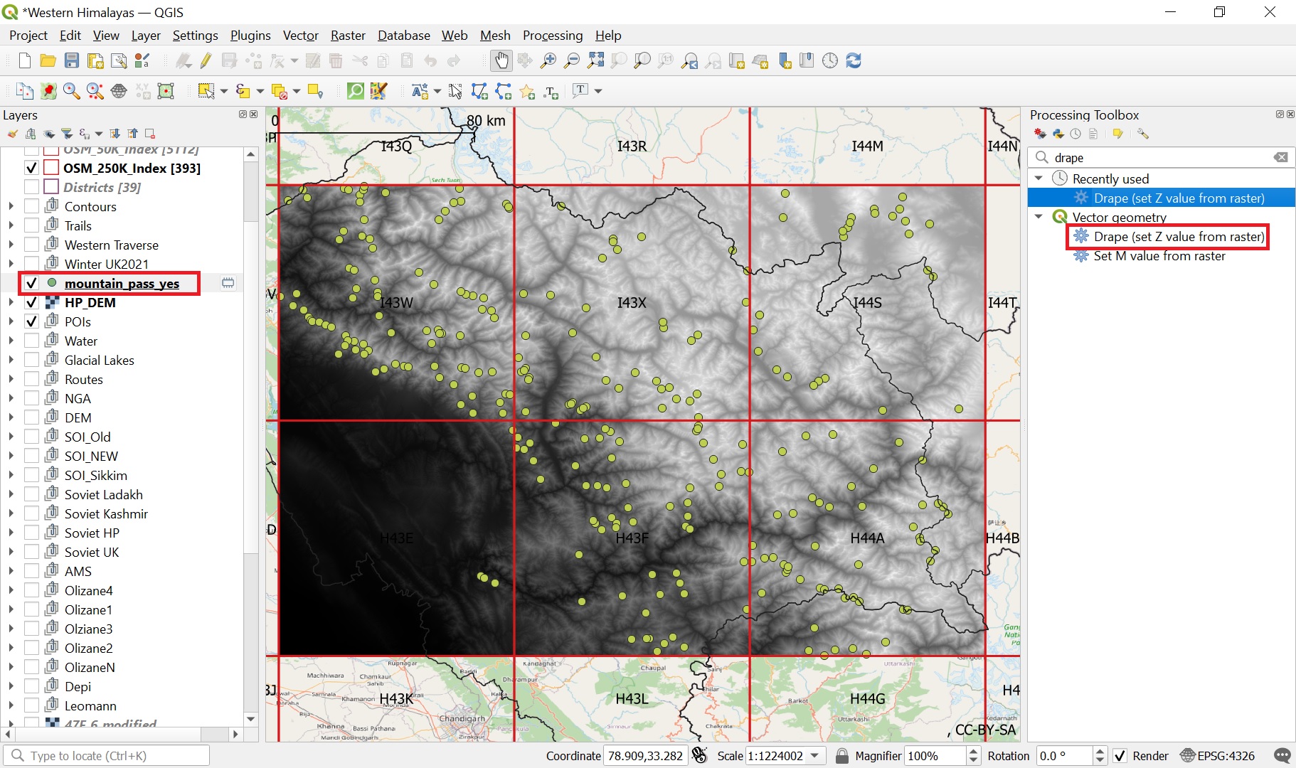
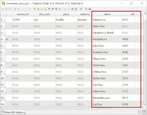
Approximately 271 mountain passes will be downloaded in a new vector layer and shown in the main QGIS window. Right click on the new vector layer and choose “Open Attribute Table” to examine the downloaded attributes. Various OSM specific fields including name and elevation (for some only) are listed. See Images 2+3 below.
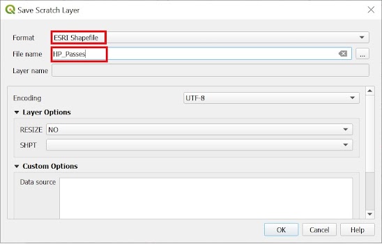
Finally, export the downloaded mountain passes as an ESRI shapefile. See Image 4 below.Querying mountain passes from Open Street Maps
271 mountain passes in 2×3 degree region covering most of Himachal
Attribute of OSM downloaded mountain passes
Exporting downloaded mountain passes as ESRI Shapefile
Extracting elevation
In this section we will extract the elevation for the downloaded mountain passes from the downloaded DEM in order to visualize and classify passes as per their altitude (useful while planning traverses as per seasons).
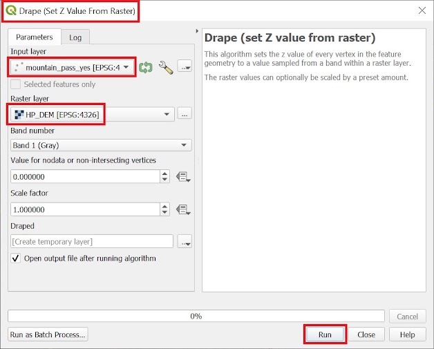
Bring up the “Processing Panel” (menu “View”, “Panels”, “Processing Toolbox”) and select “Drape (set Z value from raster)” tool. Set “Input Layer” = “mountain_pass_yes” vector layer and “raster layer” = “HP_DEM”. A new vector layer “draped” is created where the elevation corresponding to (x,y) location of each mountain pass has now been added as the “z value” (altitude, part of its geometry). See Image 1 below.
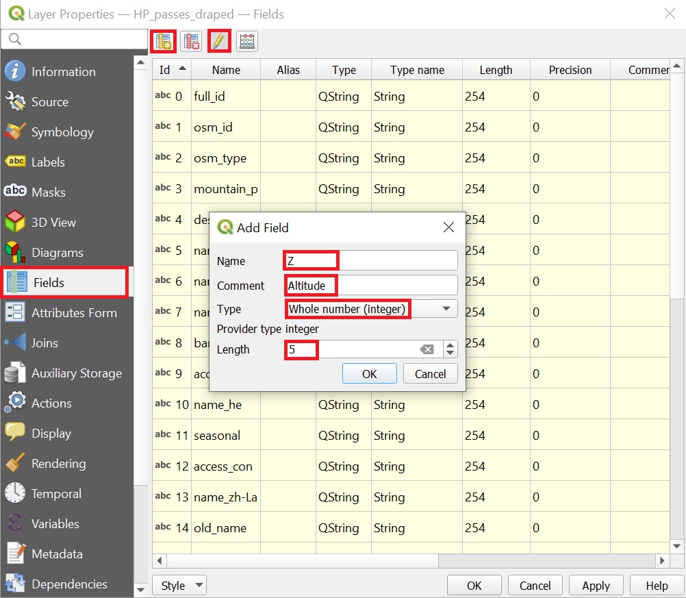
We can also extract this “z value” as a new attribute in the vector layer. Right click on the “draped” layer, select the “Fields” tab, click “Toggle Edit Mode” and “New Field” icons on toolbar. Provide a name “Z” (any name will do), comment, type and size. See Image 2 below.
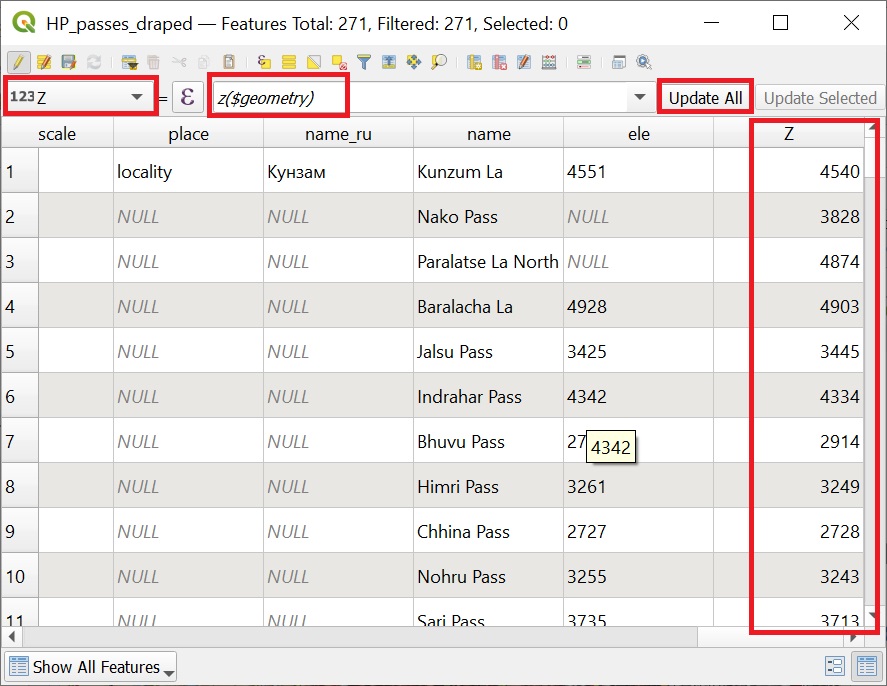
Right click on the “draped” passes, select “Open Attribute Table” and scroll to the right to see the newly added attribute. Values for this new attribute are NULL by default. Let’s now automatically update this new attribute with the extracted elevation of each pass.
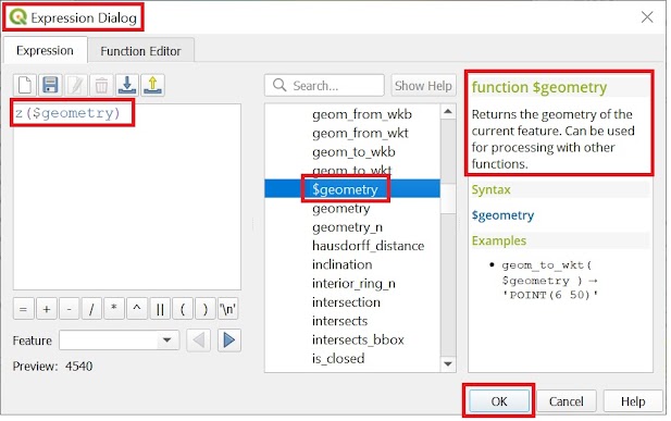
Select the new attribute in the top left combo. Click on the “E” icon to bring up the “Expression Editor”. In the “Geometry” category select the function “$geometry” to return the geometry of the currently selected feature (mountain pass). Next use the “z()” function to retrieve the “z value”. See Image 3 below.
Click “OK” to bring the expression “z($geometry)” in the value box and click “Update All” to update the newly added attribute to the altitude of geometry of current mountain pass. See Image 4 below.
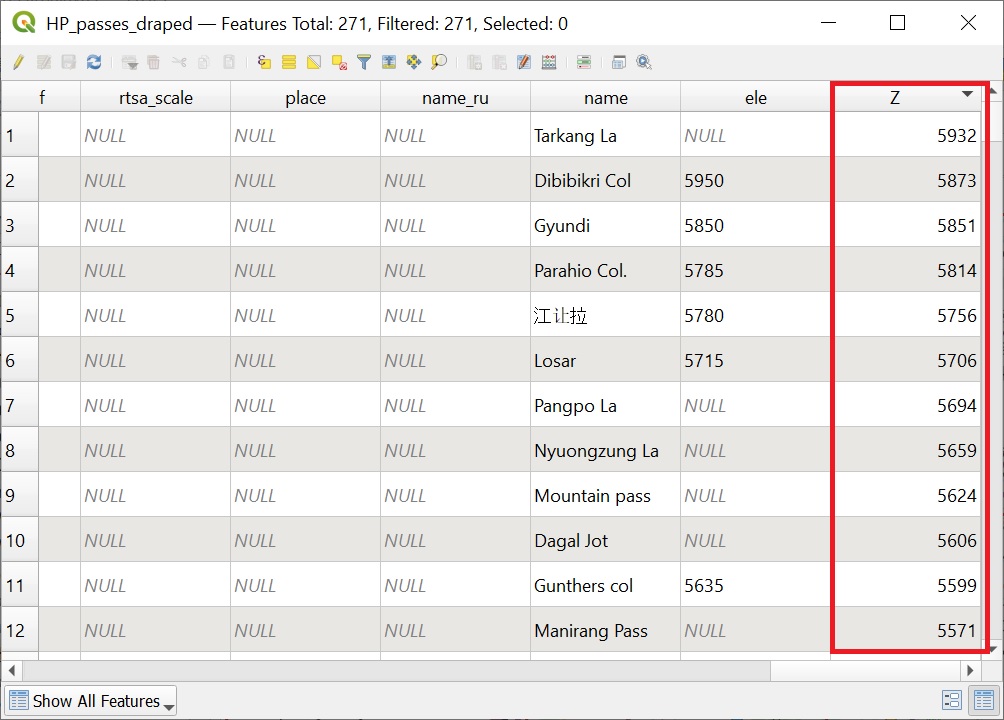
You can now see the altitude displayed in the new attribute for each pass. Click on the column of the new attribute to sort mountain passes as per their altitude. See Image 5 below.Extracting elevation from DEM for given downloaded mountain passes
Adding a new attribute to a vector layer
Retrieving the z value (elevation) from the geometry of the current feature
Updating the Z attribute with the altitude of the current feature
Mountain passes sorted by altitude
Visualizing Passes
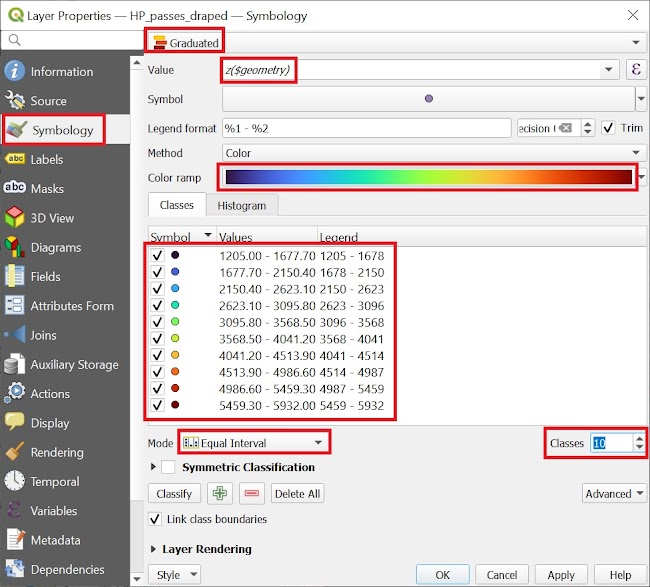
Right click on the “draped” vector layer and choose “Properties”. Select the “Symbology” tab to change the visualization of the passes as per their elevation.
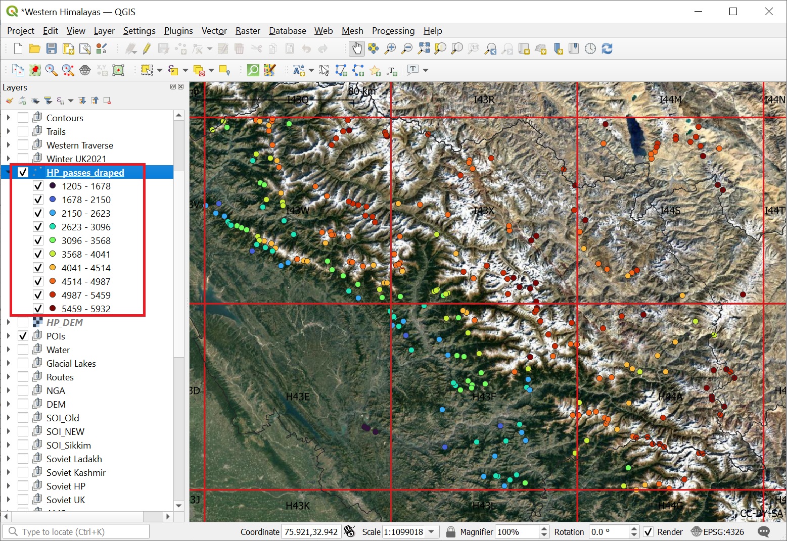
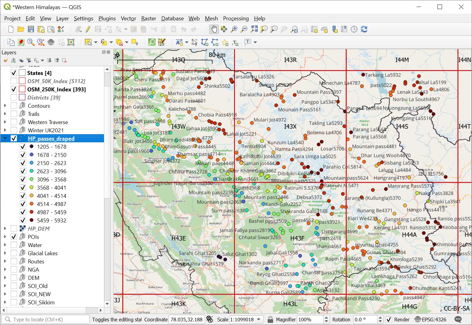
Choose “Graduated” (scale), “Value” = “z($geometry)”, “Mode” = “Equal Interval”, “Classes” = “10” and “Color Ramp” = “Turbo” (color spectrum). This will visualize passes as 10 different colors from the Turbo color spectrum (blue = lowest, red = highest). See Images 1+2 below.
Finally, let’s label the passes as per their name along with elevation. In the “Labels” tab set “Value” = “concat(name, z($geometry))” and “Size” = “8”. Concatenate name and altitude in one string. We now see the name and elevation of each pass displayed on a standard OSM base map. See Images 3+4 below.
Visualizing mountain passes as per elevation of their geometry
Mountain passes visualized as per their altitude using a color spectrum (blue lowest to red highest) on a Google Satellite basemap
Setting Label of mountain passes as name followed by elevation
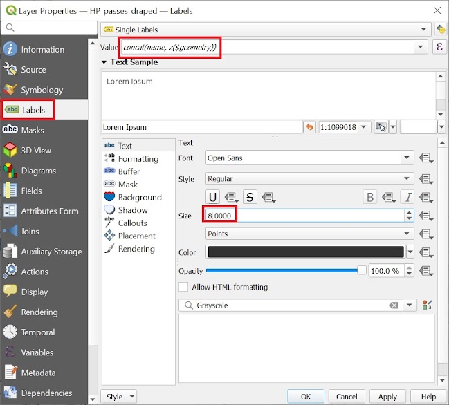
Name and altitude of mountain passes shown on a standard Open Street Map baselayer
Traverse Planning
Now consider we wish to plan a traverse in the spring season (May month) focusing on passes below 4000 meters altitude (snow free).
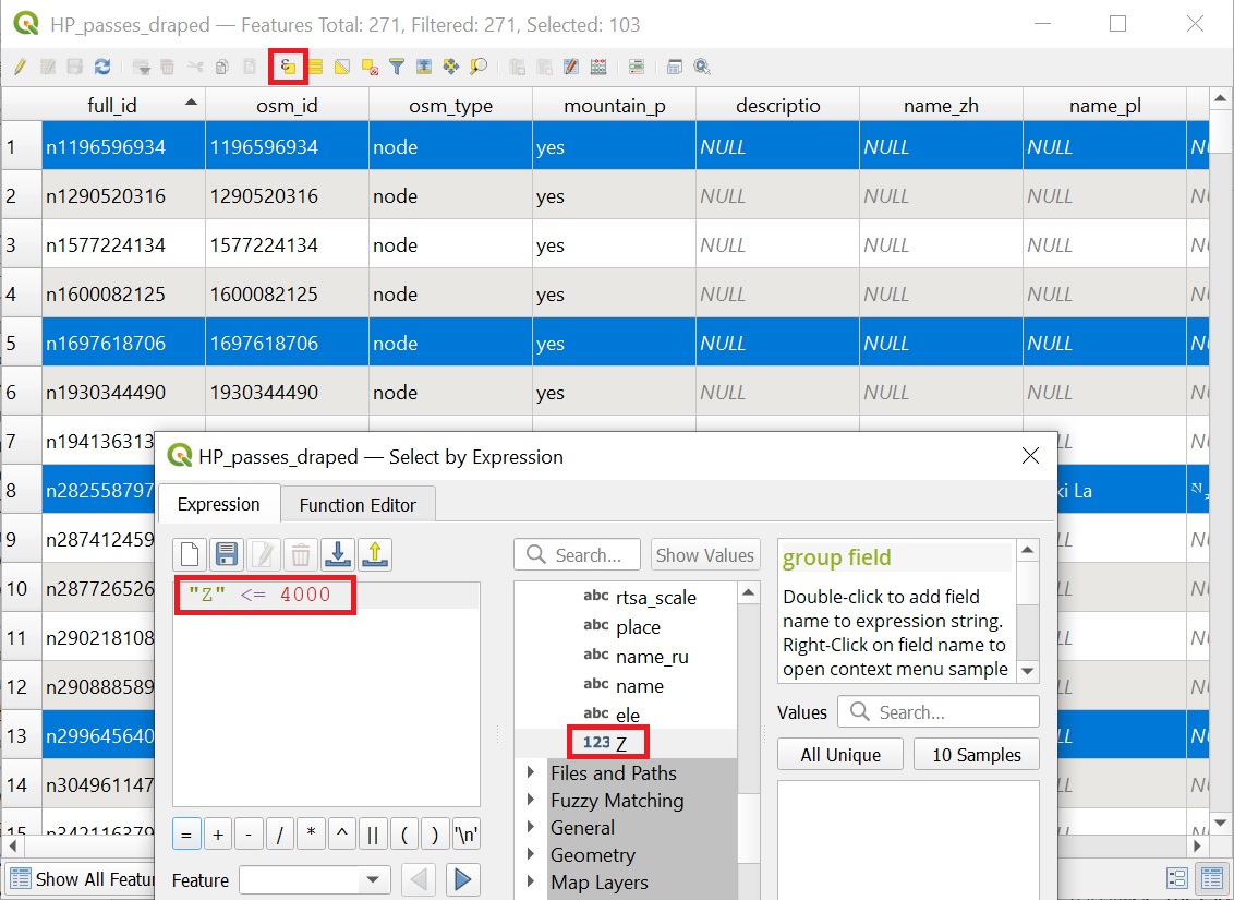
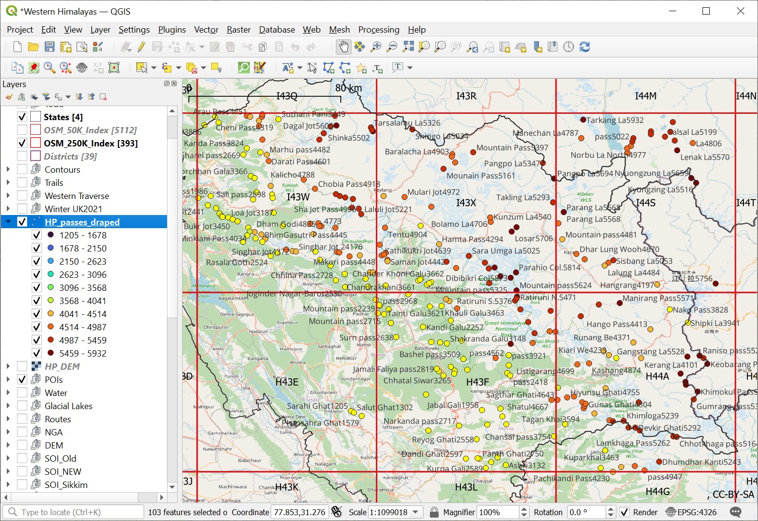
Right click on the “draped” vector layer and bring up the “Open Attribute Table”. Select the “Select features using an expression” icon from the toolbar and enter “Expression” = “Z <= 4000” (Z being the name of the newly added attribute) to select all passes with an altitude of maximum 4000 meters. See Image 1 below.
The QGIS main window will now highlight all passes below 4000 meters in yellow allowing us to plan a traverse across passes which will be free of snow in the month of May.Select all mountain passes with max altitude 4000m or less
Selected passes (altitude <=4000m) highlighted in yellow on an OSM base map
Visualizing through Charts
We can also comprehensively visualize data in QGIS using various types of charts (plots). Select the “Bar Plot” function in the “Processing Toolbox” and set “Input layer” to draped passes vector layer and “Value field” to “Z” (newly added attribute). See Image 1 below.
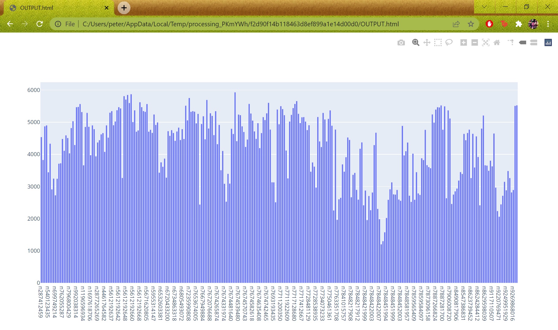
Click “Run” to generate a bar chart showing the altitude of all 271 mountain passes in Himachal. Click on “Bar Plot” in the Processing Toolbox “Results Viewer” to view the chart. See Image 2 below.
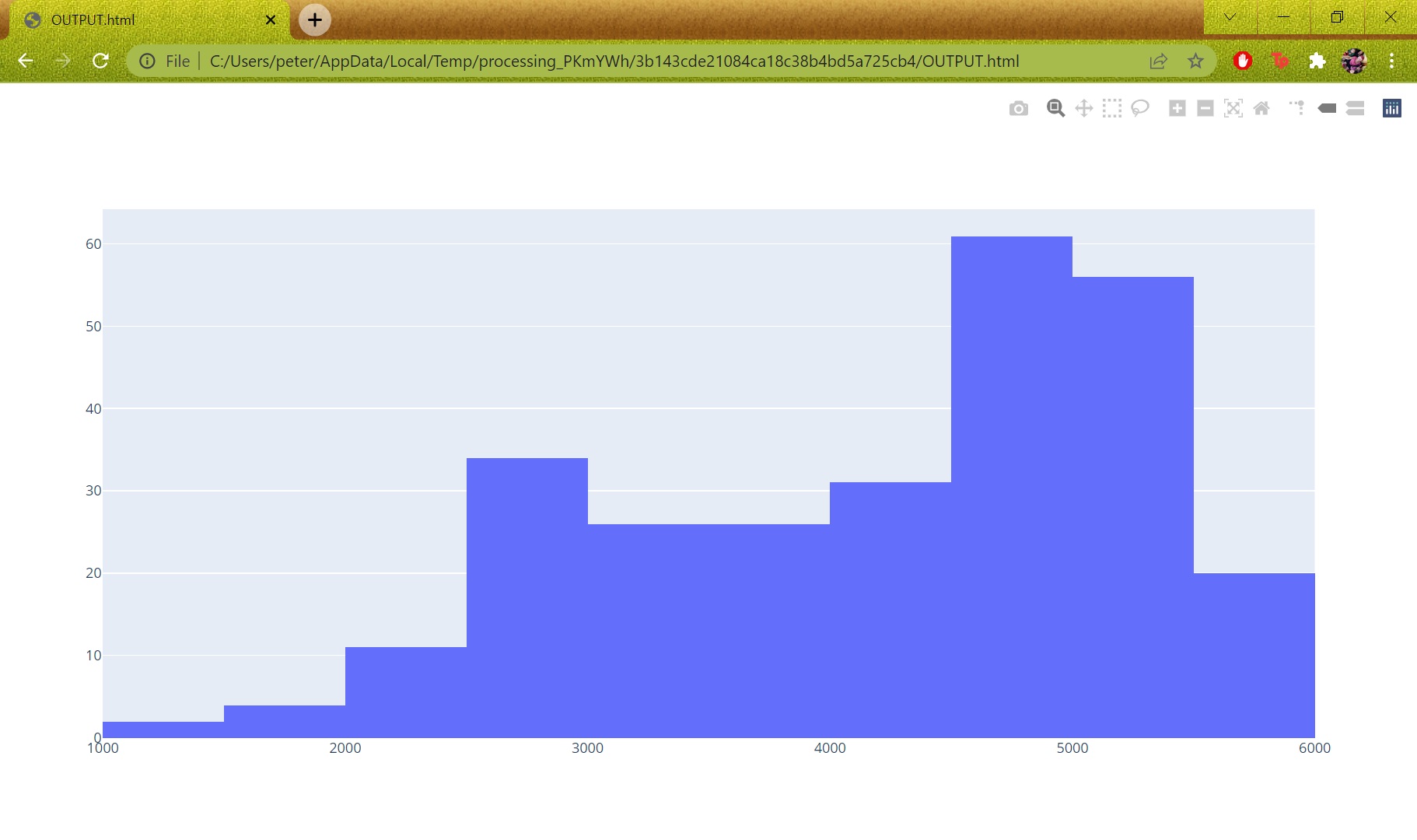
Similarly we can create a “Vector Layer Histogram” plot with “Attribute” “Z” and “Number of bins” “10” to show a histogram chart of the altitudes of passes – e.g. number of passes for each range of elevation. E.g. 32 passes have an altitude between 4000-4500m altitude. See Image 3 below.Creating a bar plot showing the altitude of the mountain passes in HP
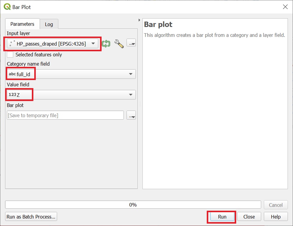
Chart showing elevation of 271 passes in Himachal
Histogram chart showing the number of passes with elevation between 1000-1500-2000-2500-etc. altitude
Assignment
Acknowledge your understanding of the concepts learned in this module by submitting the assignment below.