
Introduction
In this chapter we will teach you how to perform various interesting types of terrain analysis:
- Base Map & Projection
- Target Region & High resolution DEM (elevation)
- Contours (low scale topography)
- Hill shades (high scale topography)
- Aspect (slope direction)
- Slope (steepness)
- Terrain features
- Watershed analysis (valleys)
- Stream network
- Delineation (Catchment area)
- Ridges (inverted DEM)
Previous GIS chapters over here
Base Map
To do different types of terrain analysis we will use a comprehensive topographic base map: Thunderforest Landscape (refer chapter 1 – XYZ layer: https://tile.thunderforest.com/landscape/{z}/{x}/{y}.png?apikey=13a1166ab21c48b1a1fe90f8399cf89f )

Coordinate Reference System
The default QGIS CRS is EPSG4326 WGS 84 which uses acr degrees (1 deg = 60 nautical miles) as unit of measurement. We will instead use the UTM (Universal Transverse Mercator) projected reference system which uses meters as unit which is a more comprehensive unit of measurement. Our region used in this chapter is Manali which is located in UTM zone 43 North:

Open up Project Properties, CRS tab, search for 43N and set the project CRS to EPSG32643 – WGS 84 / UTM zone 43N:

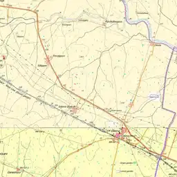
Target Region
In this chapter we will do different types of terrain analysis for the region Southwest of Manali around the Sanjoin Nal and Khanpari Khad valleys draining the Dhauladhar range in the West towards the Beas river valley in the East:

High resolution DEM
To do terrain analysis we require DEM – Digital Elevation Data. Standard DEM has a resolution of 30m which misses smaller topographic details. The NASA EarthData ASF Data Search Vertex site provides 12 meter DEM which allows us to do more accurate terrain analysis. Refer below post on how to download 12m DEM:
For our target region you can simply download hires DEM directly over here:
https://drive.google.com/file/d/1KIEwJjLeH67AoQpD2tfnZ9K9H3Erb05D/view?usp=sharing

Drag n drop the DEM (Geo TIF format) file into QGIS and it will open as a raster layer showing elevations from 546 meters (black) to 6066 meters (white) altitude. A gray scale is used to show lower regions as darker and higher altitude areas in lighter shades. We can also show the changes in elevation more comprehensive using a spectrum of multiple colors. Go to the layer Properties – Symbology and change Render Type from Singleband Gray to Singleband Pseudocolor:

This will show the transitions between different elevations as a color spectrum from blue (low) – green – yellow – orange – red (high) allowing us to distinguish regions of different elevations: Beas and Paravthi river valleys are shown as blue, the Dhauladhar and Pir Panjal high ranges West in red:

To start our terrain analysis we will focus on a smaller region as the most terrain processing functions are time (CPU) consuming on larger regions. Let’s clip the above DEM data to our target region. Select the DEM raster layer and choose Raster – Extract – Clip Raster by Extent.

For the Clipping Extent choose Draw on Map Canvas to select the target region:

A new DEM raster layer is created as shown below:

Contours
Topographic maps will show the topography as contours – lines that connect points of equal elevation. We can generate contours from DEM. Select the clipped DEM layer and choose Raster – Extraction – Contour menu. A default contour interval of 10 meters can be changed to the desired contour interval.

Un-thick the other layers and zoom into a scale of 5-10K to clearly view the 10m contour lines. The density and shape of contours allows us to identify important terrain features such as steepness, peaks, valleys, ridges and more. Refer the alpine bootcamp course (chapter 1.2) for more details.

Hill Shades
Where contours help us to understand the lower scale topography, hill shades give us insight in macro topography by adding shadows using a virtual light source just like the sun adds light and shades to the real-world terrain around us. Choose Processing – ToolBox and search for the Hillshade funtion:

Run the Hillshade function with default parameters:

A new raster layer is created which shows hill shades clearly revealing ridgelines, valleys and in-between slopes.

Hill shades are best viewed when combined with another baselayer. Select the hill shades raster layer and choose Properties – Transparency – Set Global Opacity to 30%

Viewing both contours and hill shades (30%) layers gives a comprehensive view on the topography at a scale of 10K.

To view a larger region we can use a higher contour interval say 100m at scale 100K giving an insight in the overall topography of the region:

Contours and hill shades can be used to add topography to basemaps. For example the standard Open Street Maps looks flat:

Overlaying contour lines and adding hill shades creates a proper topographic map:

Aspect
Terrain aspect, in geography, refers to the direction a slope faces, measured in degrees from 0 to 360, with 0 being north, 90 being east, 180 being south, and 270 being west. Use the Raster – Analysis – Aspect function to generate a new raster layer which represents the Aspect for our target region:

Say we wish to identify all North facing slopes where we are likely to encounter more snow while hiking. We can simply identify all points where the the Aspect is less than 90 or more than 270 degrees. Choose Raster – Raster Calculator::

This generates a new raster layer which shows all North facing slopes as white and the remaining in black.

We can improve the visualization by changing the Symbology to Render Type = Paletted / Unique values. Choose Classify to choose two colors for both values (1 = North facing, 0 = Others).

In the Transparency tab add ‘0’ as Additional NoData value to make the other slopes invisible.

This now highlights all North facing slopes in yellow or whatever color you choose for value 1 (Aspect <= 90 or Aspect >= 270):

Slope
Terrain slope, also known as gradient or incline, refers to the steepness or angle of a land surface relative to a horizontal plane. It’s a crucial aspect of terrain analysis, impacting various aspects of natural and human environments. Use Raster – Analysis – Slope to generate a new raster layer that shows the gradient of the terrain between 0 (flat) and 75% (very steep):

We can improve Slope visualization by choosing a SingleBand pseudocolor with Mode = Equal Interval and Classes = 10 to show highlight 10 slopes with increasing steepness in 10 different colors:

Showing both Contours and Slopes we can see a clear correlation between contour spacing and steepness of the terrain. Closely spaces contours are steep regions (red). Widely spaced contours correspond to flatter slopes (blue).

Say we wish to identify slopes with gradient of less than 30 degrees which would be suitable for step cultivation. Choose Raster – Raster Calculator and ‘Slope”1 <= 30’ to identify the same

All slopes with gradient less than 30 degrees are now shown in white:

We can improve visualization in Symbology by setting Render type = Paletted/Unique values, choose appropriate colors and set Transparency – Additional NoData value as ‘1’ to hide steeper slopes:


Bringing up a satellite map (Web – QuickMapServices – Bing – Areal) we can see that human settlements and cultivation mostly happens on these lesser steep slopes:

Overlay Survey Map clearly shows the cultivated regions (yellow) correspond to slopes with lesser gradient (<= 30 degrees).

Survey map can be added as an XYZ layer:

With URL: https://indianopenmaps.fly.dev/soi/osm/{z}/{x}/{y}.webp

Terrain Features
Using DEM we can identify various terrain features like peaks, ridges, valleys, saddles and more. Terrain features can be easily identified on topographic maps by analyzing the shape of contours further visually assisted by hill shades. Terrain features are identified by their relation to the surrounding landscape comparing the difference in elevation:

Filling Sinks
For further terrain analysis we will be using various processing functions of the SARA NextGen Provider plug-in. Go to Plugins menu and search for ‘Processing Saga NextGen Provider’ and select Install to add the plugin to QGIS

First we need to ensure there are no sinks in our DEM (often introduced due to limited resolution of DEM). Choose the Saga – Fill sinks (wang & lue) function in the processing toolbox


Un-check the Flow Directions and Watershed Basins layers and only keep the ‘Filled DEM’ while running the Fill function:

A new Filled DEM layer is created which has a slightly different elevation range as the original Clipped Region

For all further analysis we will be using this ‘Filled DEM” raster layer.
Watershed Analysis
Watershed analysis allows us to identify valleys and basins (rivers and catchment areas). We will be using the SAGA Strahler order function to identify the stream network based in our target region using the Filled DEM data. Strahler assigns orders to stream as illustrated below – initial gullies are number ‘1’. Two gullies joining into a stream ‘2’. Two streams ‘2’ join a bigger stream ‘3’. Lower order streams joining higher order streams do not change the order.

Ordering streams allows us to easily filter out smaller streams and only view the major rivers are valleys. Let’s run the Strahler Order SAGA function on the Filled DEM and we get a new raster layer as shown below identifying streams of order 1 to 10:

We can visualize this stream network better using Symbology=Paletted/Unique values, Classify, Transparency Additional NoData value=’1′ (smallest streams). Still this results in quite a massive drainage network:

Let’s extract only the larger streams. Use the Raster Calculator to select streams of order 6 and above.

Let’s enhance the visualization of the resulting layer by Render Type = Paletted/Unique values and Transparency Additional NoData value = ‘0’.

The raster layer now clearly visualizes all major streams of Strahler order 6 and above:

Stream Network
The Strahler Order function generate raster files. To generate metrics for our stream network its easier to work with vector files. Run the ‘Channel Network and drainage basins’ SAGA function in the processing toolbox.

Use the ‘Filled DEM’ as input raster for elevation. Set threshold equal to Strahler order 6. Enable only Subbasins and Channels. Order layers can be disabled

A vector layer is generated (line type) representing our stream network.

Open the Attribute Table to view the individual stream segments including order and length in meters.

Use the Expression editor to generate metrics. For example the total length of all streams in our target region is 358km.

We can enhance the visualization by choosing Symbology – Categorized, Value = ‘ORDER’, Classify to view different order stream segments in different colors.

This visualizes stream segments in 6 different colors as per the Strahler order.

Delineation (catchment)
Let’s now identify the drainage basin or valley or catchment area for a given stream. Let’s say we wish to identify the basin for all water that flows through below point:

Enable the Strahler_gt6 raster layer, zoom in and right click on the exact point on the stream from which to calculate the catchment area.

Invoke the SAGA Upslope Area function in the processing toolbox. Copy the X/Y coordinates of the point. Select the Filled DEM as the elevation raster.

This will generate a new raster layer showing the catchment area for the stream flowing through the given point.

We can convert this raster to a polygon using the Raster – Conversion – Polygonize (Raster to Vector) menu.

A new vector layer is created using one polygon identifying the catchment area

Open the Attribute Table and choose Field Calculator to add a new field

Add a new field ‘area’ and set it as ‘$area / 10^6’ or the area of the catchment in square kilometer

The total size of the catchment area is 133 square kilometers

Change the Symbology to Inverted Polygon – White color

This hides everything outside the catchment area while showing the stream network inside

Change the Symbology of Channels vector layer to Single Symbol – Blue – 0.5 Width

Viewing the Stream Network for the given catchment are with 100m contours and hill shades over the original elevation colored DEM shows as:

Ridgelines
Ridgelines and Valleys are opposite terrain features. To identify ridgelines we can use the same functions after inverting the DEM. Open up the Raster Calculator on the Clipped DEM layer and use “Clipped_DEM@1” * -1

A new inverted DEM layer is created showing high areas (ridges) as dark and low areas (valleys) as light, the opposite of the original DEM layer.

Before doing terrain analysis through SAGA functions we again need to fill up sinks by running the ‘Fill Sinks (Wang & Liu)’ processing function on the Inverted DEM. Watershed Basins option can be un-checked.

Now execute the SAGA ‘Channel Network and Drainage Basins’ function in the processing toolbox. Use ‘Filled_Inverted_DEM’ as Elevation. Set Threshold as 6 (Stralher order). Enable only the Channels output.

A new vector layer ‘Channels’ is created based on inverted DEM which actual corresponds to ridgelines now.

Viewing the inverted channels on 100m contours and hill shades clearly confirms the topography of the ridgelines –

Finally we can visualize both streams and ridges on a shaded basemap clearly showing the topography of the terrain:
