
QGIS is a powerful GIS software. In Chapter 6 we learned how to import and visualize geo-tagged alpine lakes, query passes and hiking routes from Open Street Maps, geo-reference maps, download DEM data and generate contours and generate map tiles for offline navigation.
In Chapter 8 we familiarized ourselves with various map sources for the Western Indian Himalayas, digitize trails and settlements, compare and analyze accuracy of various maps. In Chapter 9 we will generate a district-wise atlas of the Western Himalayas visualizing key features like passes, peaks and alpine lakes.
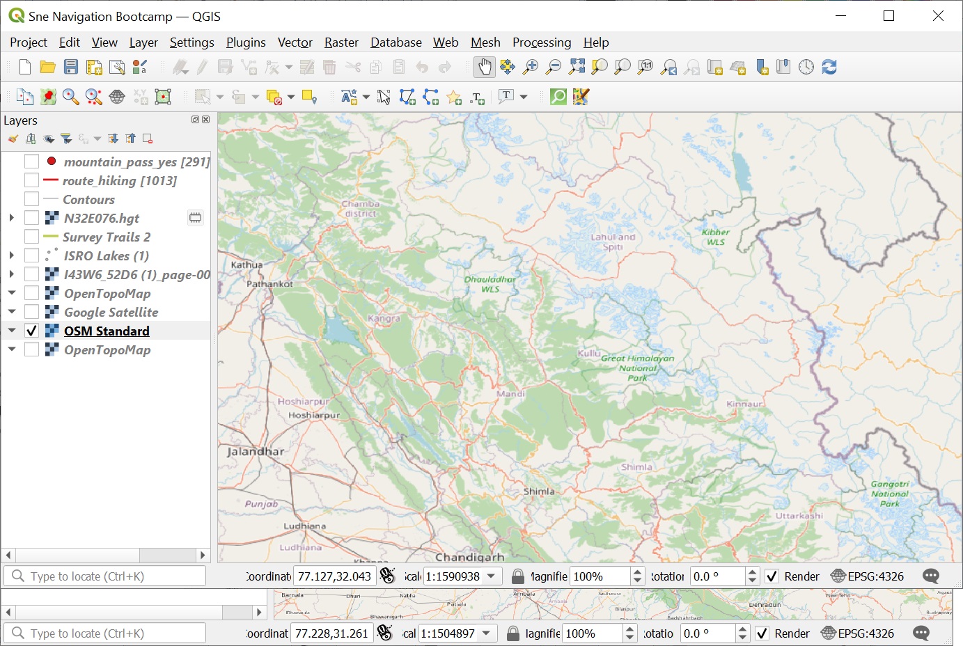
Open up QGIS and zoom to a scale of 1:1500000 centered around Himachal. This should partly show the 4 Western Himalayan states – J&K, Ladakh, Himachal and Uttarakhand. See Image 1 below.
States
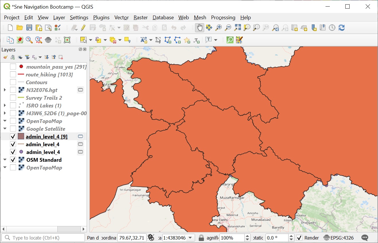
Let’s query the OSM states intersecting with our current QGIS view. A “state” is usually tagged in OSM as “place=state”. However in case of India we can use “admin_level=4”. Open up “Quick OSM” plugin and run a query on the current canvas window. Around 9 intersecting states will be returned as polygons in a new vector layer. See Image 1 below.
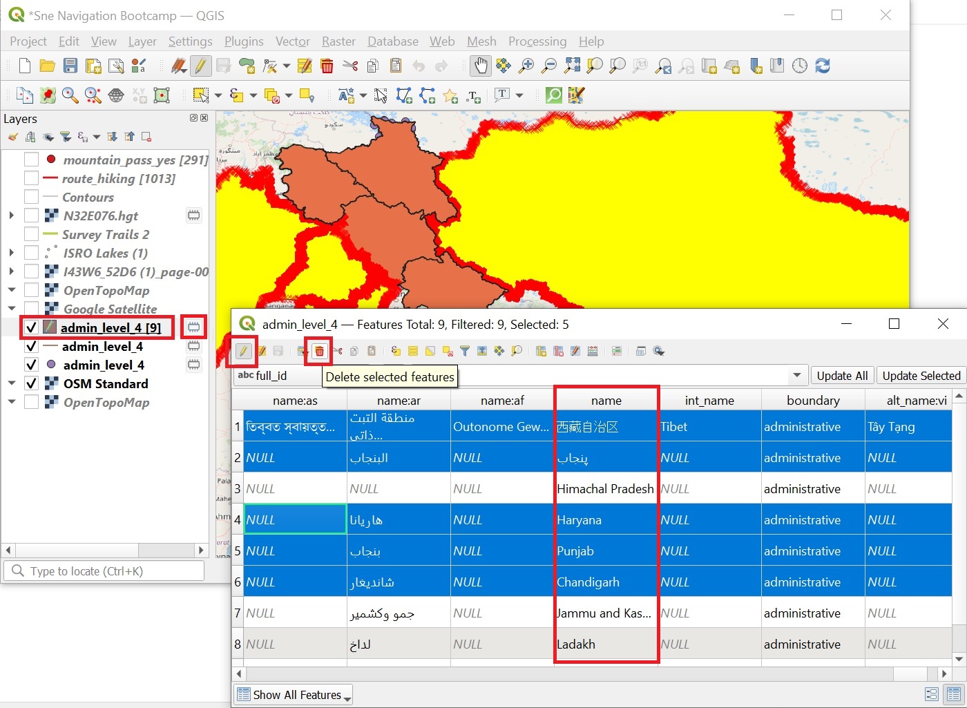
Right click on the layer and select “Open Attribute Table” to view all the states returned (“name” column). Click “Toggle Edit Mode” icon, select the non-relevant states and select “Delete Selected Features” icon to retain only “Himachal”, “Uttarakhand”, “Ladakh”, “Jammu and Kashmir”. See Image 2 below.
Rename the vector layer as “Himalayan States” and click the memory icon next to the name to save the layer as an ESRI shapefile.
Districts
Similar as above, let’s query the Himalayan districts (“admin_level=5”) through the “Quick OSM” plug-in. Ensure the QGIS map window just includes the 4 Himalayan states and run the query using the current canvas.
All districts partly intersecting with the current view will be returned (around 120) as a new shapefile vector layer. See Image 1 below.
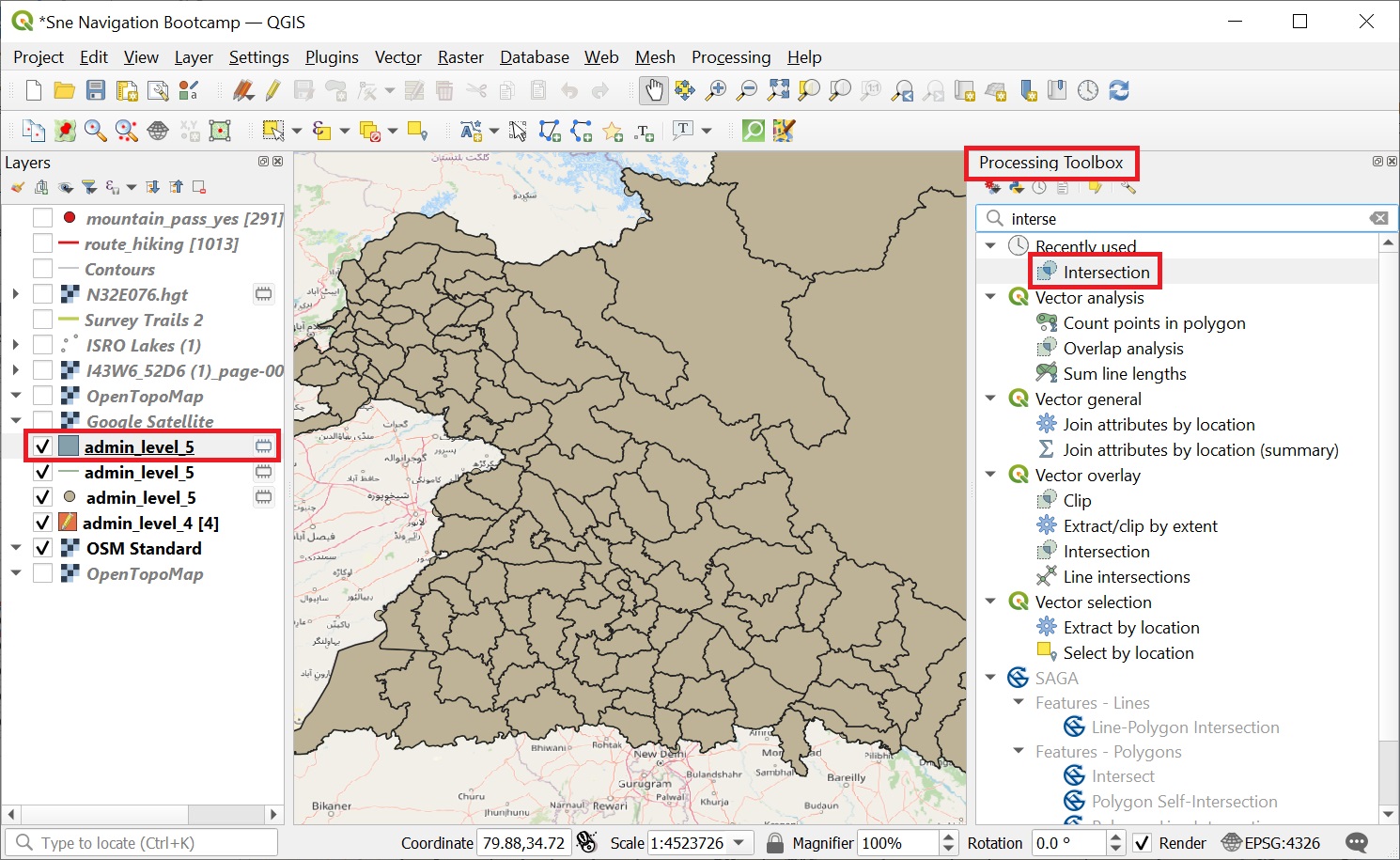
Select the newly created layer and choose “Intersection” from either the “Processing Toolbox”
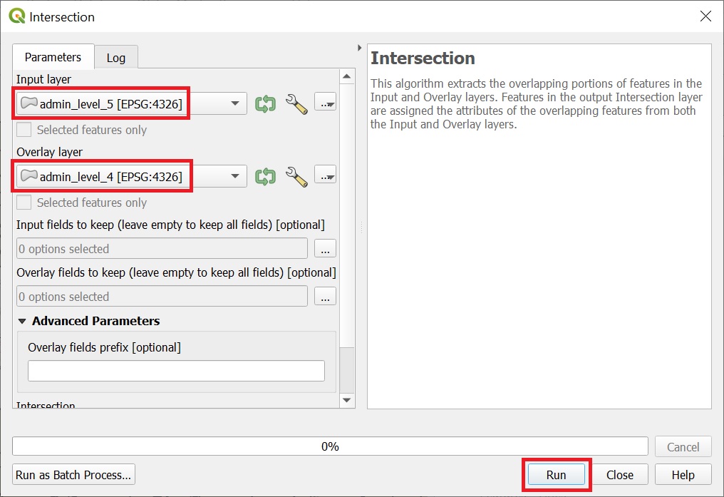
We can now do an “Intersection” of the returned districts within the 4 Himalayan states. Choose “Intersection” from either the “Processing Toolbox” or the “Vector” / “Geoprocessing” menu. Ensure the districts are selected in the “Input” layer and the states are selected in the “Overlay Layer”. See Image 2 below.
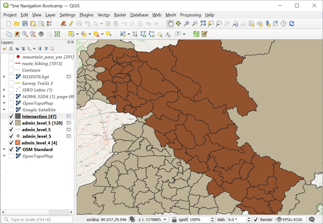
Run the “Intersection” operation and you will get 47 districts returned in a new vector shapefile layer which are part of the 4 Himalayan states. Delete the original vector layer (120 districts) and rename / save the new vector layer (47 districts) as an ESRI shapefile. See Image 3 below.
Visualization
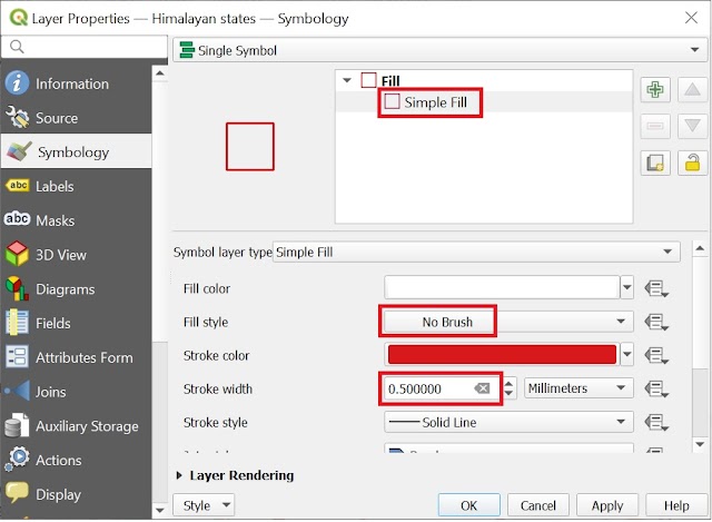
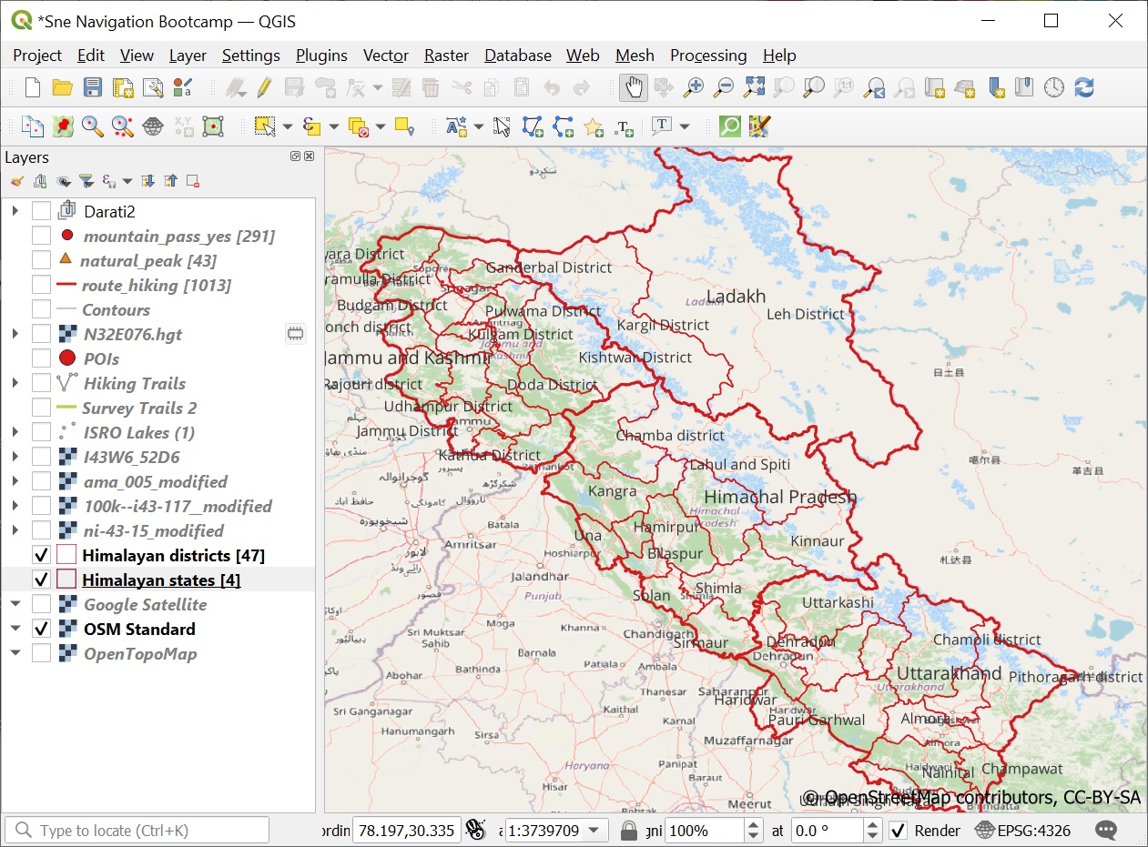
Finally, let’s provide a comprehensive visualization for the Himalayan states and Districts. Right click on both layers, choose “Properties” and in “Symbology” chose “Fill style=No Brush”, “Stroke color=red”, “Stroke width=0.5” (states) or 0.25 (districts). This will show the districts as as transparent polygons (underlaying base map remains visible) with only the borders visible. See Image 1+2 below.
Under “Labels” select “Single Label” and chose OSM “Name”.
Assignment
Acknowledge your understanding of the concepts learned in this module by submitting the form below